In many fields of computer graphics, randomly sampling a mesh’s surface is an important step. Sometimes, you may want to create a random sample across several meshes. This article introduces a simple, performant, and effective way to sample the surface of a mesh. These algorithms have applications in remeshing, point-based graphics, texturing, and next event estimation (Shirley 2022, Šik 2013).
Personally, I am researching this topic to implement next event estimation in my path tracer, which I have spent the past two months developing. More advanced techniques use hierarchical light sampling, but simpler, easier-to-implement approaches utilize random point sampling on a mesh’s surface (Shirley 2022, Tokuyoshi 2024). I am writing this article because there are few resources on this subject found when googling “how to randomly sample the surface of a mesh,” or similar terms. I hope that this article will reach those who search for similar terms in the future.
Prior work discusses how to sample points on a mesh according to a probability density specified by a 2D image (Šik 2013). This is perfect if you want to use different noise functions, such as blue noise or perlin noise, but implementing this method probably is not worth the time if uniform sampling is suitable. Chapter 16 of the Ray Tracing Gems book describes how to uniformly sample a mesh (Shirley 2019). However, the approach described in that book can be simplified further.
In this article, I will describe a naïve approach to randomly sample a mesh, explain why the naïve approach doesn’t work, describe a corrected algorithm to uniformly sample the surface of a mesh, then validate the algorithm by testing for bias. I will also discuss how this algorithm can be extended to uniformly sampling multiple meshes. I will use Python-like pseudocode for this article with the intention that someone familiar with any language can understand it and implement it in their language of choice. Real Python code is also provided at my GitHub repository.
A naïve approach might be to pick a random triangle in a mesh, then pick a random point on that triangle. You could do something like this.
def get_tri_vertices(vertices, indices, tri_idx):
    """
    Given a triangle index, get the vertices of that triangle
    """

    i0 = indices[tri_idx * 3 + 0]
    i1 = indices[tri_idx * 3 + 1]
    i2 = indices[tri_idx * 3 + 2]

    v0 = vertices[i0]
    v1 = vertices[i1]
    v2 = vertices[i2]

    return v0, v1, v2

def sample_mesh_naive(vertices, indices):
    # random integer between [0, int(indices_length / 3) - 1]
    rand_triangle = randint(0, int(len(indices) / 3) - 1)

    # get the triangle vertices for that triangle index
    v0, v1, v2 = get_tri_vertices(vertices, indices, rand_triangle)

    # sample a random point on the triangle
    return random_sample_triangle(v0, v1, v2)
The above code chooses a random number between \([0, \lfloor \frac{\text{len(indices)}}{3}\rfloor - 1]\) because, in a mesh, every three consecutive indices make up one triangle. The additional \(-1\) is to avoid off-by-one errors causing the index to be out of bounds.
random_sample_triangle is a function that returns a
random point on a triangle given its 3D coordinates. It maps two random
points in a unit square to a triangle, then converts those points from
barycentric space to world space given the triangle vertices. This is
described in Ray Tracing Gems chapter 16 (Shirley
2019).
def random_sample_triangle(v0, v1, v2):
    # random() generates a random number in the range [0, 1)
    beta = 1 - sqrt(random())
    gamma = (1 - beta) * random()
    alpha = 1 - beta - gamma

    return alpha * v0 + beta * v1 + gamma * v2  # convert to world space
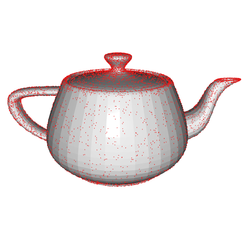
Below we see the output of this algorithm with 10,000 random points
on the famous Utah teapot mesh. The red points are samples chosen using
the naive approach. However, there’s a very large flaw with this
algorithm. 
This is more evident if we increase the sample count to 1,000,000:
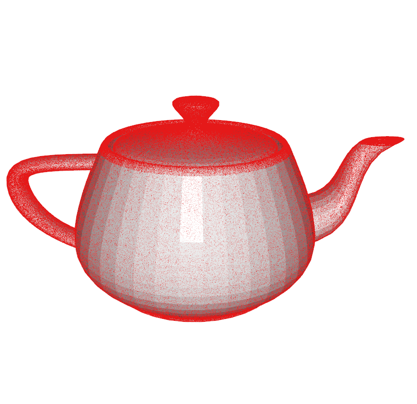
Areas on the teapot that are made up of larger triangles have fewer samples, while areas that have smaller triangles have more samples. This is inherent to how we designed our algorithm: we chose a triangle randomly, regardless of area.
For the application of next event estimation, this approach can work, considering note that the probability of a random point being chosen (which you will later learn is the PDF) is described as: \[P(N, A) = \frac{1}{NA}\] Where \(N\) is the number of triangles and \(A\) is the surface area of the selected triangle. It’s important to note that this solution will likely converge slower than if we were to use a corrected algorithm, however.
To fix this issue, it’s helpful to have a basic understanding of the probability density function (PDF) and cumulative density function (CDF). If you already have grasp of these concepts, you can skip to the “A Better Approach” section.
The probability density function (PDF) describes the probability that a randomly-sampled value taking on a particular value. Since a PDF is for continuous values, we need to instead describe the probability of the sample within a range. For example, if that range is \([a, b]\), then we can express it as: \[P(a \leq X \leq b) = \int_a^bf(x)dx\]
One key characteristic about PDFs is that they are normalized, meaning the total area under the curve of the PDF is 1. This can be described mathematically as: \[\int_{-\infty}^{\infty} f(x)dx = 1\]
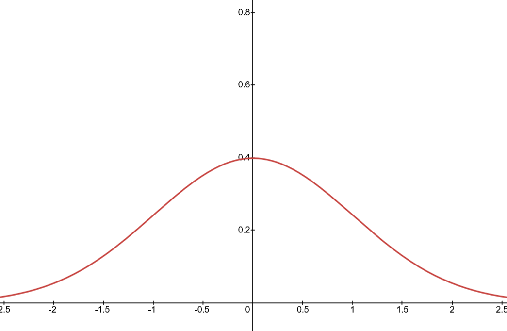
One of the most famous PDFs is the Gaussian distribution (a.k.a. the normal distribution), which is given by a scary-looking – and for our purposes, irrelevant – formula. However, you may recognize the graph:
The cumulative density function (CDF) is an extention of the PDF. It describes the probability that a uniformly distributed sample \(u < x\) given a PDF \(f\). \[F(x) = \int_{-\infty}^x f(t) dt\]
For the Gaussian distribution, you can see how this creates a sigmoid-like curve. Notice that this function will always be ordered (that is, \(f(x_1) < f(x_2)\) if \(x_1 < x_2\)).
You can use a CDF to sample any PDF by mapping a uniformly
distributed random number from \([0,
1]\) (such as the one returned from random(), or
similar random functions) to the PDF. To do this, you can perform binary
search on the CDF.
Below is an example in code. Notice that the CDF is discrete and presented as an array. This will be helpful with the implementation of the better sampling approach later on. To adjust the previously-shown formulas to their discrete versions, you can replace the intergral with a summation.
This function takes in a cdf parameter (array of
floats), and a rand parameter (a random float between \([0, 1)\)).
def sample_cdf(cdf, rand):
    # Binary search algorithm to find the index in cdf
    # with the closest value to the rand parameter
    lower_bound = 0
    upper_bound = len(cdf) - 1

    while lower_bound <= upper_bound:
        midpoint = (lower_bound + upper_bound) // 2

        if cdf[midpoint] < rand:
            lower_bound = midpoint + 1
        elif cdf[midpoint] > rand:
            upper_bound = midpoint - 1
        else:  # due to the continuous nature of the rand variable, this is very unlikely
            return midpoint

return lower_boundThe question we’re asking, “how to uniformly sample a mesh,” can be expanded to “how to sample a mesh such that the density of points is constant across all areas of the mesh.” Therefore, the probability that a point will be inside surface area \(n\) given that the mesh has surface area \(N\) can be computed as:
\[P(\text{point in area n}) = \frac{n}{N}\]
If we define these “areas” on the mesh (\(n\)) as the triangle areas, then we can construct a PDF and CDF of the mesh. Technically, since the PDF is discrete with one probability value for every triangle, the correct term is a probability mass function (PMF).
The revised algorithm can be simplified into three steps: 1. As a preprocessing step, create the PDF then the CDF for the mesh. 2. Sample a uniform random
We can actually skip a step by computing its CDF directly, instead of computing the PDF then CDF. This saves us a bit of work.
def generate_cdf(vertices, indices):
    cumulative_area = 0
    cdf = []  # in an actual implementation it is recommended to preallocate int(len(indices) / 3) zeros

    for tri_idx in range(int(len(indices) / 3)):
        # get_tri_vertices is defined in the naive approach section
        v0, v1, v2 = get_tri_vertices(vertices, indices, tri_idx)

        area = 0.5 * length(cross(v1 - v0, v2 - v0))
        cumulative_area += area
        cdf.append(cumulative_area)

    # normalize the CDF
    for idx in range(len(cdf)):
        cdf[idx] /= cumulative_area

    return cdf
The algorithm above collects the cumulative area of a triangle over
all triangle indices and stores it in the cdf list. Then,
it normalizes the CDF by dividing all elements by the total area of the
mesh (which cumulative_area is equal to after it is done
iterating). The algorithm also uses the fact that the area of a triangle
is equal to \(\frac{1}{2}
\|(\overrightarrow{v_1 v_0} \times \overrightarrow{v_2
v_0})\|\).
Now that the CDF is constructed, we need a way to sample a mesh. We
can use the sample_cdf function from the The Cumulative Density
Function (CDF) section. This code block is simple since the required
functions are already written.
def sample_mesh(vertices, indices, cdf):
    # get the random triangle index with probability proportional to its area
    sampled = sample_cdf(cdf, random())

    # get the triangle vertices at the index
    # this function is defined in the naive approach
    v0, v1, v2 = get_tri_vertices(vertices, indices, sampled)

    # return the point randomly sampled on the triangle
    # this function is also defined in the naive approach
    return random_sample_triangle(v0, v1, v2)
If we generate 10,000 points with the new approach, we get this: 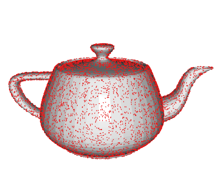
1,000,000 points yields: 
Much better! Note that it looks like there are more points near the edges, but that’s just due to perspective.
We’ve tested visually that the points are correct, but what does the math say? If we average the position of all points, it should be very close to the mesh’s area-weighted centroid. I’ll spare you the implementation details, but this can be computed like so:
\[\overrightarrow{C} = \frac{\sum_{i} A_i \overrightarrow{C_i}}{\sum_{i} A_i}\] Where \(\overrightarrow{C}\) is the area-weighted centroid, \(\overrightarrow{C_i}\) is a vector pointing to the center of the \(i\)th triangle, and \(A_i\) is the area of the \(i\)th triangle.
I then calculate a bias vector by subtracting the centroid from the average position of all points: \[\text{bias} = \frac{\sum_{j}\overrightarrow{P_j}}{j} - \overrightarrow{C}\]
Where \(\overrightarrow{P_j}\) is the \(j\)th random point generated with the revised approach and \(\overrightarrow{C}\) is the triangle centroid.
We then use the standard error of the mean (SEM) to compute the following \(\text{bias} \space \plusmn \space 1.96 \cdot \text{SEM}\). If 0 is within the range, then we do not have enough evidence that the bias is significantly different from 0. In our case, this statistical insignificance is desired since that indicates that there is no bias.
For the revised approach, we calculate the bias and SEM as:
       X Axis       Y Axis      Z Axis
Bias: [-0.0054202   0.00360548  0.00224182]
SEM:  [0.013908   0.00896356 0.01038037]
Bias values closer to 0 are better. From these values, we can therefore conclude that the revised sampling technique is unbiased.
We can also test the naïve approach’s bias:
       X Axis     Y Axis     Z Axis
Bias: [0.00267655 0.41176464 0.01097711]
SEM:  [0.01575905 0.00993715 0.00822669]
The Y value is not within the margin of error, which confirms our suspicions that the method is biased. The bias values tell us that the method is biased mostly towards the positive Y direction, but this varies per-mesh.
Expanding this algorithm to sample multiple meshes is relatively smiple. You would need to create and sample another CDF that is proportional to each mesh’s area. Then, once a mesh is selected, use the technique described in this article to sample the mesh. It is also possible to combine all meshes into one big mesh, then use the technique described in this article. However, modifying one mesh would require recalculating the entire CDF, which is more computationally expensive than recalculating the CDF for meshes only.
In this article, I aimed to introduce a simple, efficient, and unbiased approach to uniformly sample a mesh. By detailing the limitations of the naïve approach and presenting a corrected algorithm, I hope to equip you with a reliable uniform mesh sampling method for 3D mesh processing.