Introduction
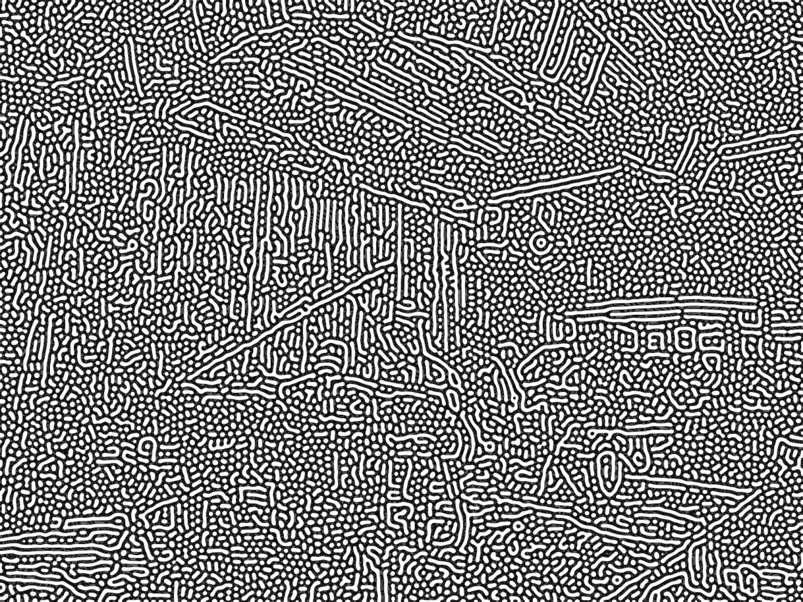
In 1952, foundational computer scientist Alan Turing introduced the Turing Pattern, formed with signals
diffusing and reacting.
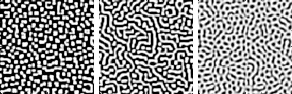 Image of three Turing patterns (Wikimedia Commons).
These patterns appear all over nature. They’re pretty obvious in pufferfish skin and cheetah fur, but have also been instrumental in developmental and mathematical biology, chemistry, physics, and ecology (Nature Computational Science Editors 2022).
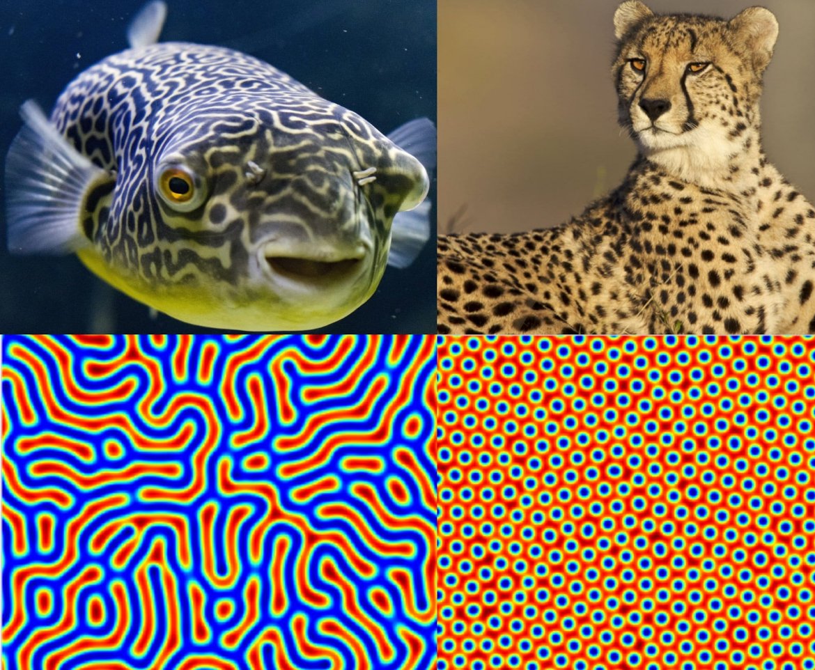 Turing patterns appearing in pufferfish and cheetah skin or fur (Chris Keegan).
I was first exposed to Turing patterns by a short YouTube video by Patrick Gillespie by titled “What Happens if You Blur and Sharpen an Image 1000 Times?” (Gillespie 2025). He described this type of reaction-diffusion pattern by sharpening and blurring images repeatedly, and generated Turing patterns that still hold a vague resemblance to the original image.
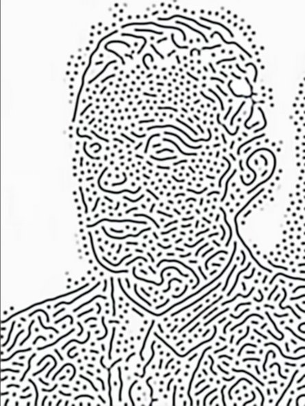 A screenshot of a Turing pattern from Gillespie's video.
Gillespie points out that he’s not the first to discover this technique. In 2015, Andrew Werth published a paper describing how sharpening and blurring an image is mathematically equivalent to a reaction-diffusion Turing pattern Werth 2015).
My Work
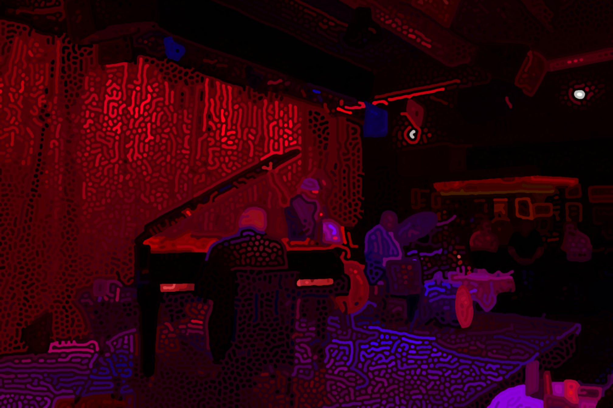
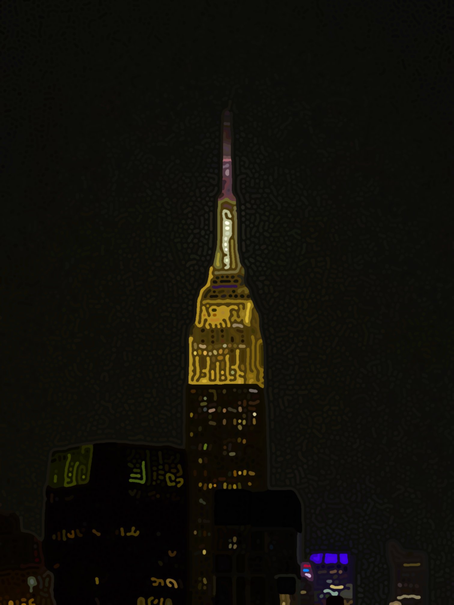
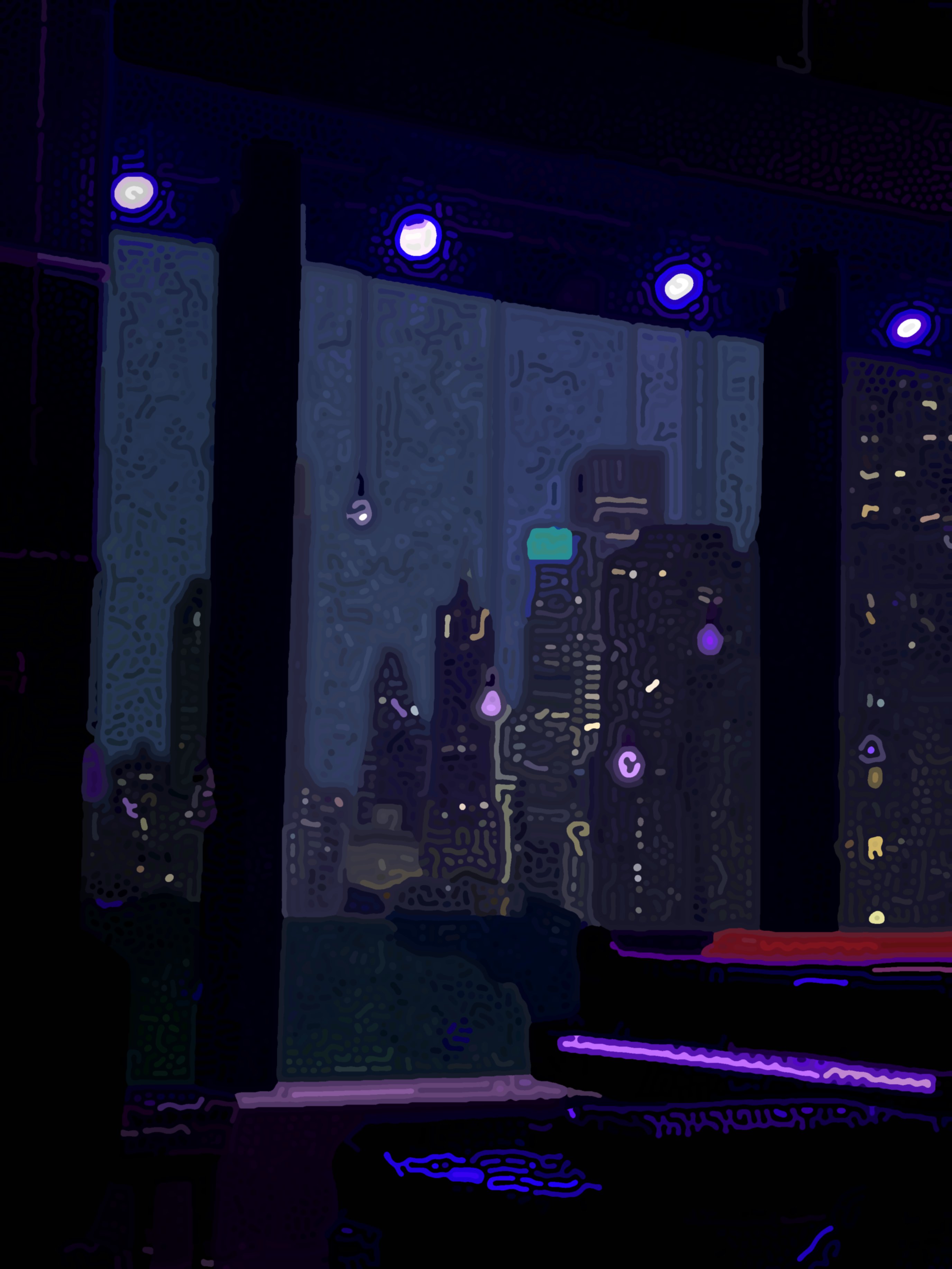
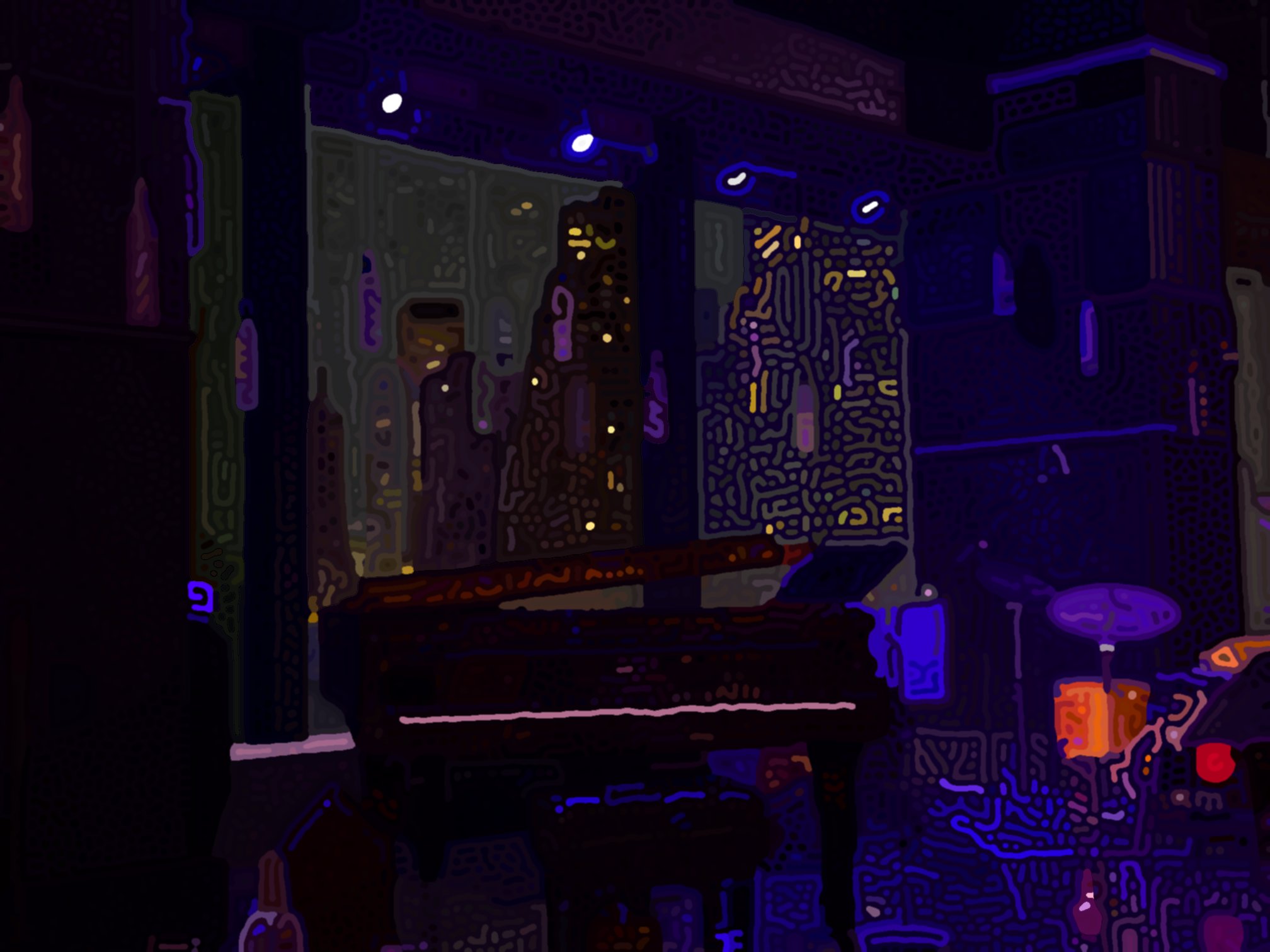
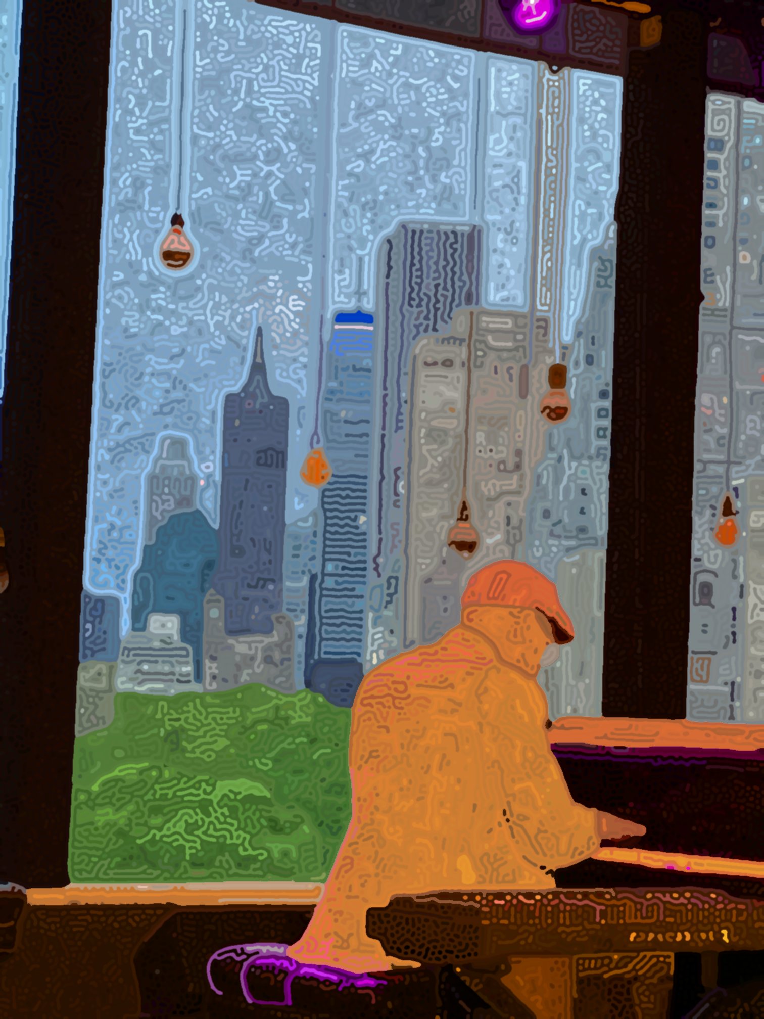
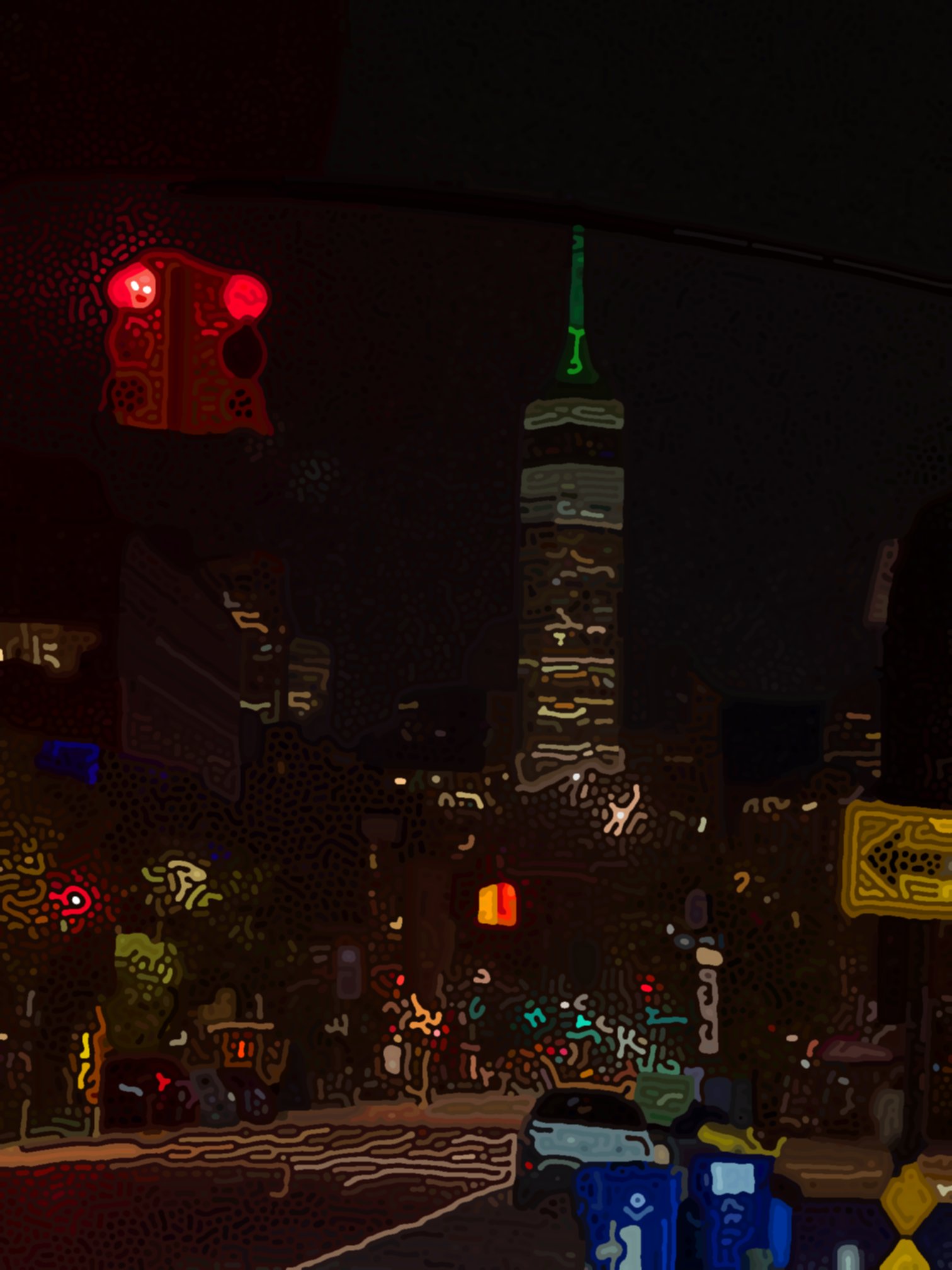
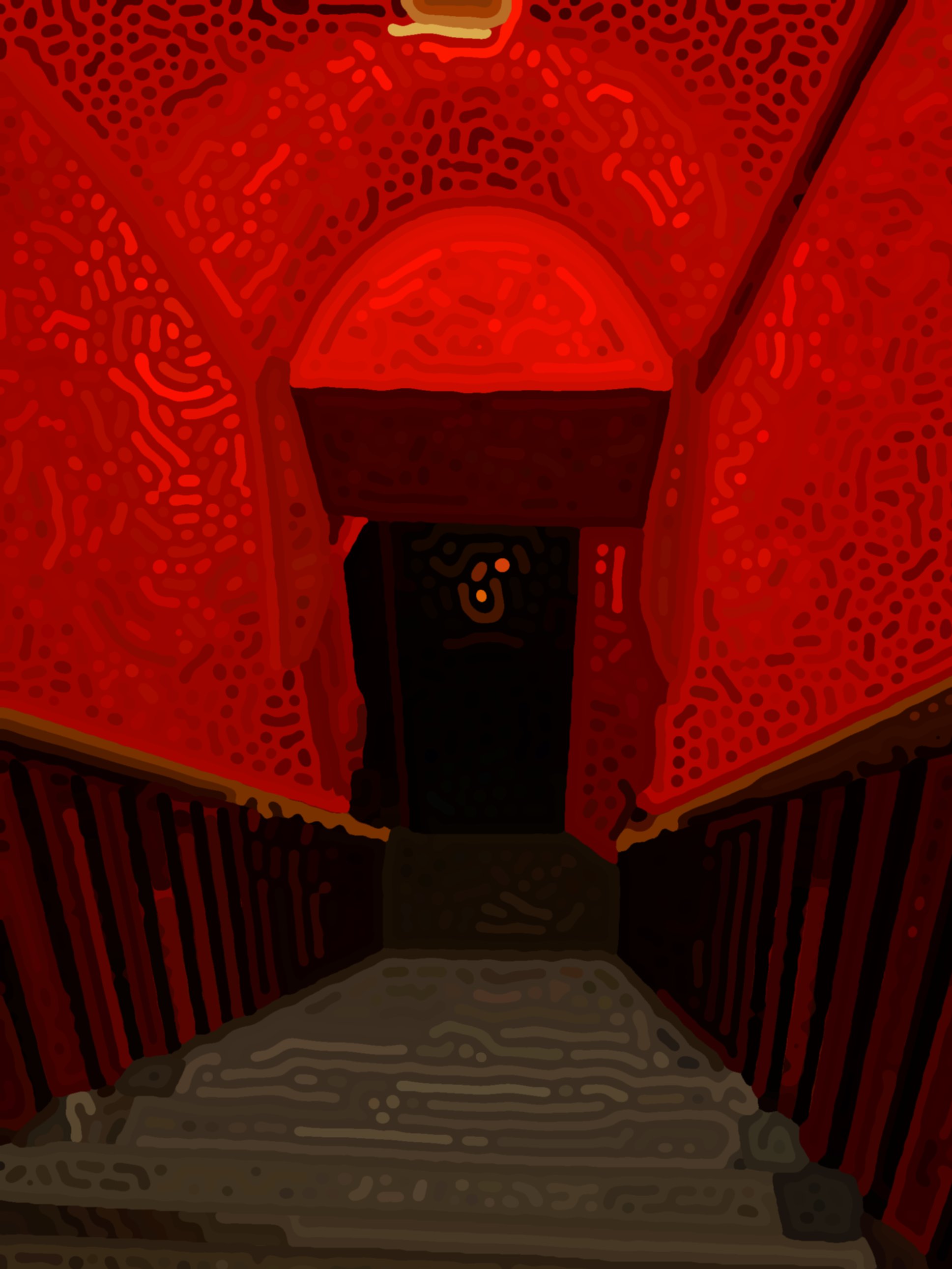
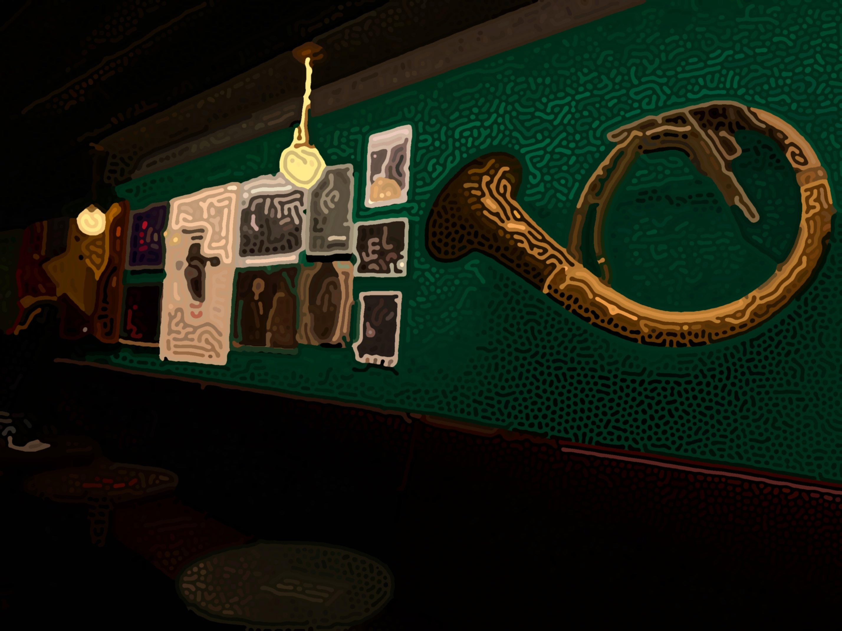
When I saw Gillespie’s video, I thought to myself: wouldn’t it be cool if these images had color? Here’s what I
created. All of these images are under the theme of New York City jazz clubs, because I found that stage
lighting works best with the algorithm and is relevant to my interest in jazz. I took the base pictures in May
2024 and July 2025.
Technical Details
An Initial Approach
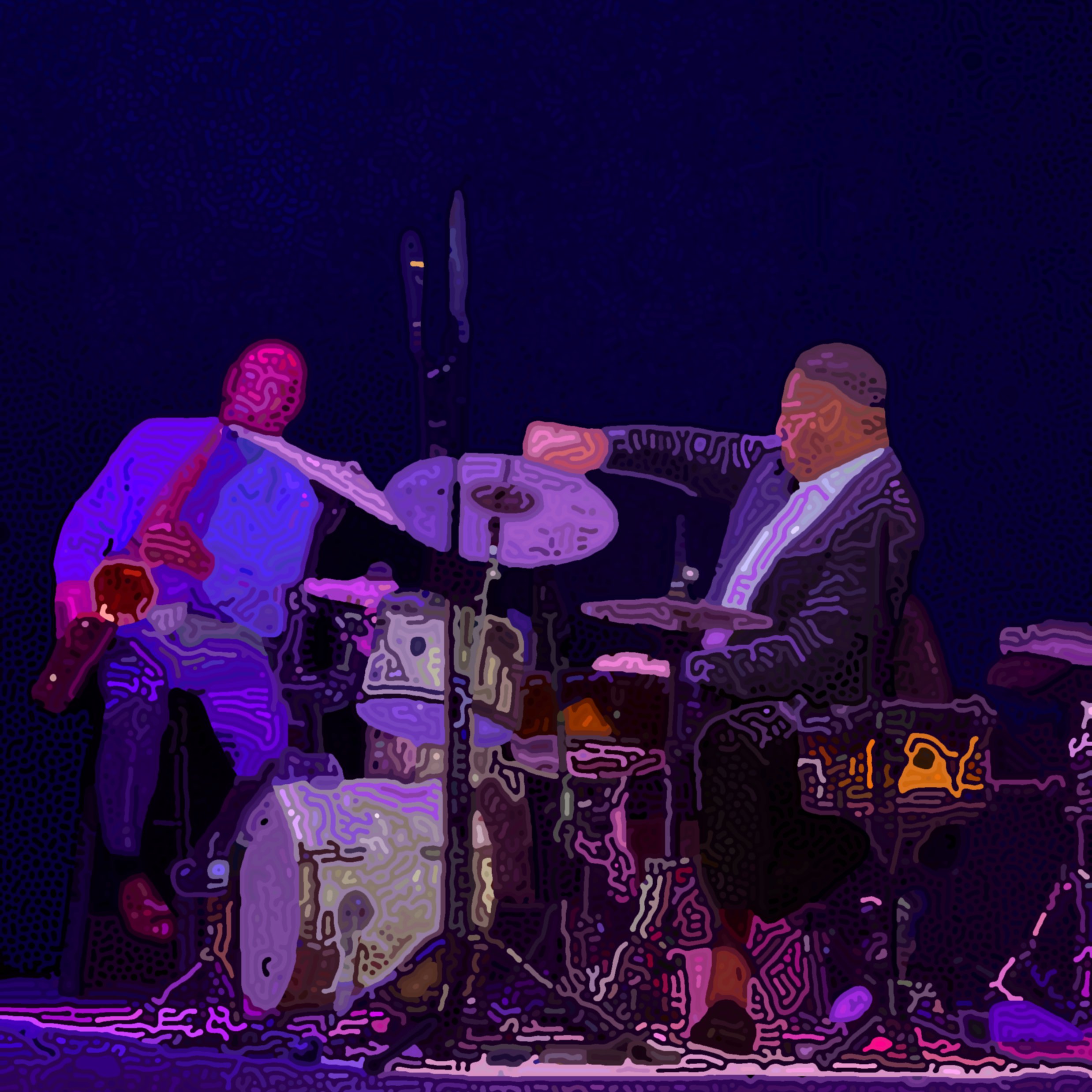
Take an initial image. I took this photo while at the Birdland Jazz Club in Manhattan.

Then, let’s blur and sharpen the image hundreds of times. I found that I get better results if I convert the
image to grayscale before running this process.
Now, let’s take a binary threshold of this image. Let’s give each black and white region a random color:
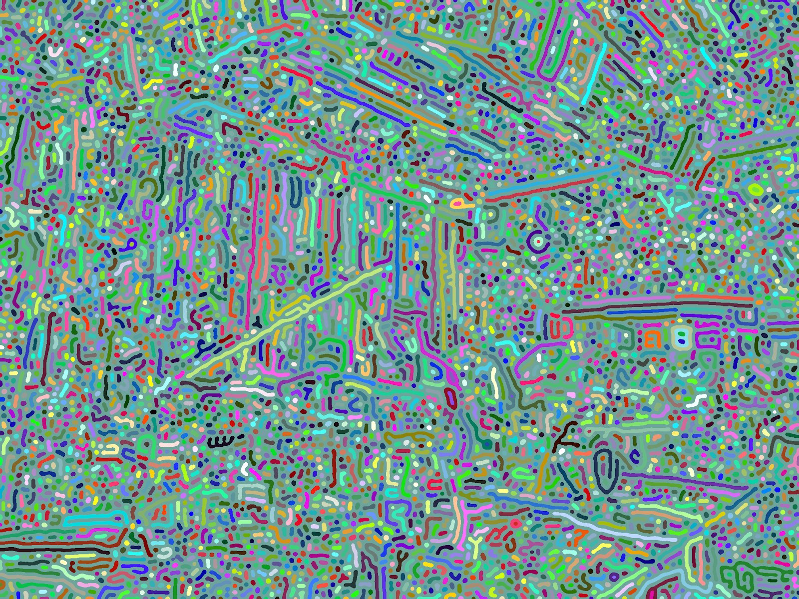
That returns an unintentionally psychedelic image, but it seems like every black and white region is being correctly identified!
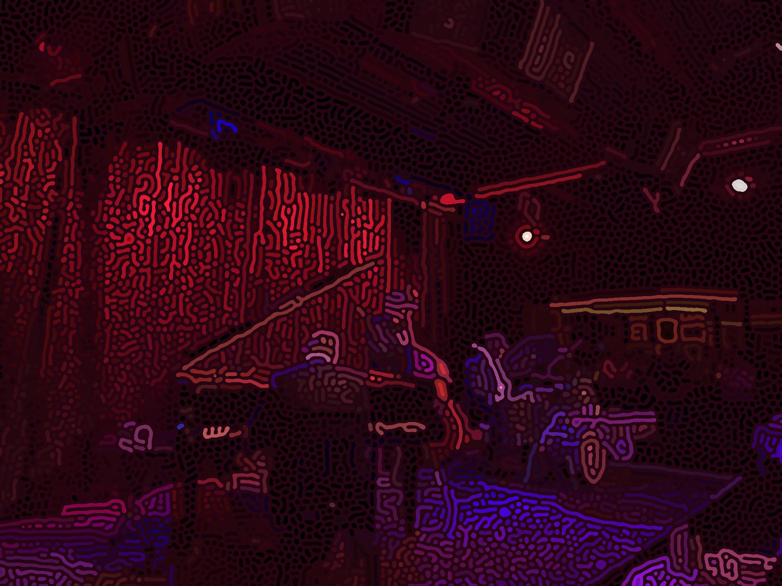
Now, instead let’s color each region based on the average color of the original image in that region’s location.

This looks really good! But it can still be improved. Most importantly, it’s somewhat hard to tell what the image depicts. If I showed you this image without showing the original image, you may identify that this is a photo of a stage with a pianist and bassist, but you may not be able to recognize details of the drummer. Additionally, the spectators in the background are almost completely gone.
Another issue is that many regions look disconnected. For example, it seems that the pianist’s head is made up of seven regions that do not touch. That’s because one interconnected, ‘monolithic’ region covers the whole image, and our current approach colors each region just one color.
I highlighted the monolithic region in
white, and all other regions in black. Notice how the black regions span only a small space of the image, but
the white region spans the entire image.
Both these issues can be solved with image segmentation.
Image Segmentation
The main idea with image segmentation is to locate different objects of the image, and apply the Turing pattern algorithm to each segment individually.
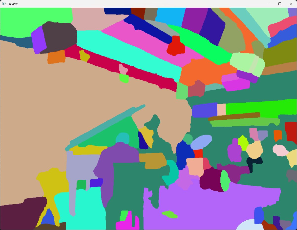
To segment the image, I use Meta’s Segment
Anything Model (SAM). After I color each class as a random color, I get this
output:
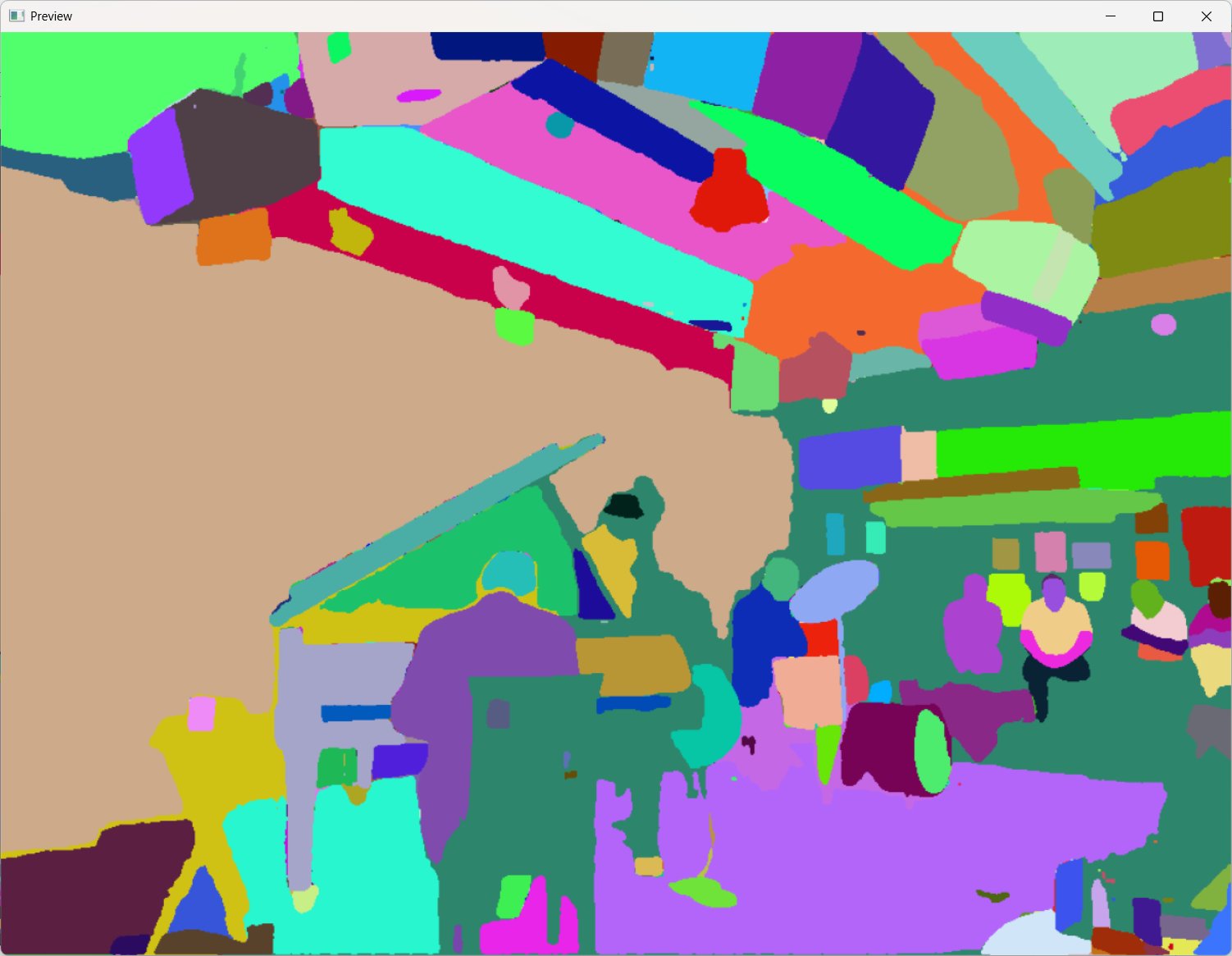
Nice! It successfully identified the main objects in the image. If we process each segment individually then put
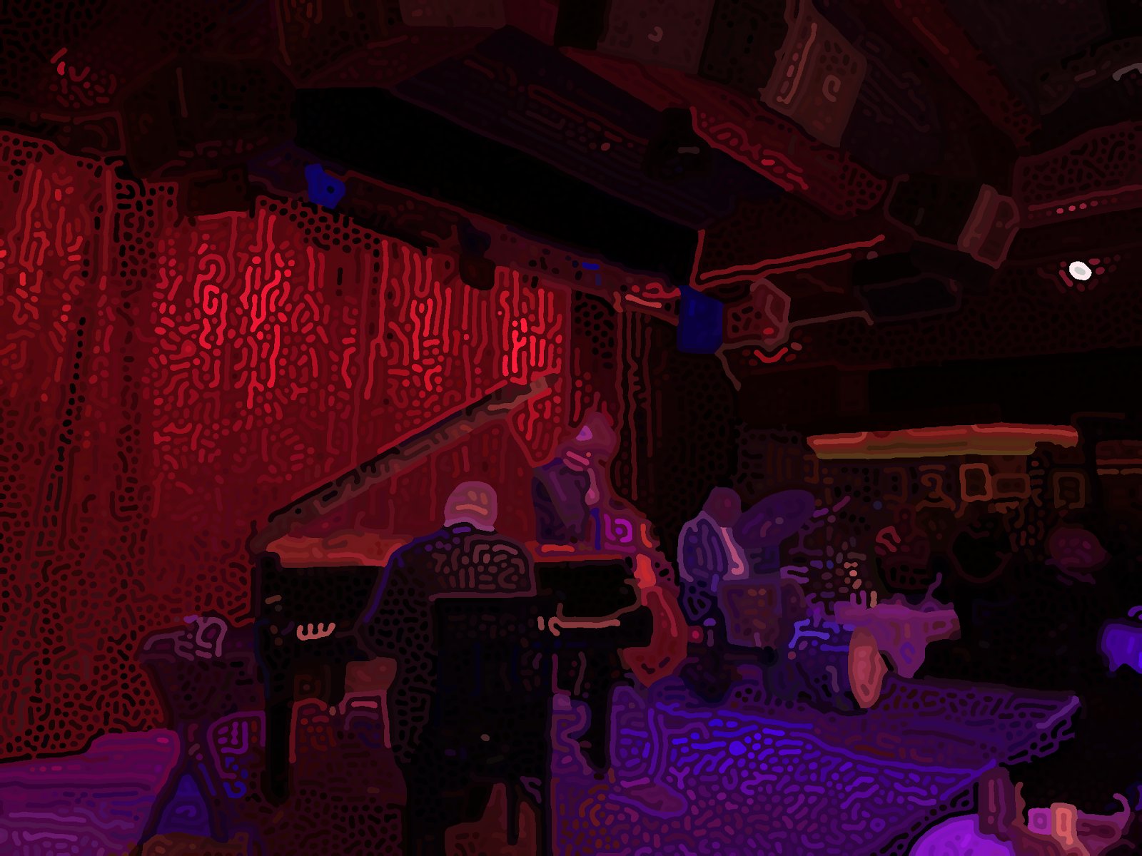
that all together in one image, we get this:
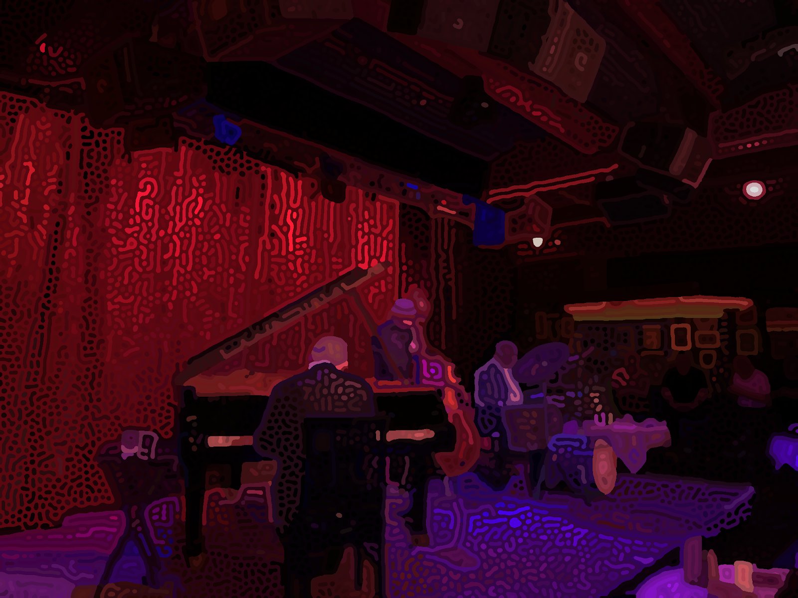
I think this is much better! Objects look more “solid” and you can see fine details like the drum kit and people
in the background. It’s not perfect, though. If you zoom in, you can see some flaws. Notably, SAM likes to
create small segmentations that shouldn’t exist, like the holes in the pianist’s chair. These sometimes create
weird splotches in the final image that look visually inconsistent. I circled some of the problematic regions in
red:
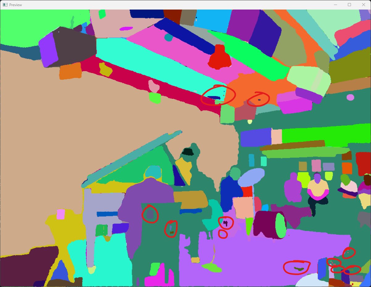
My solution to this issue is fairly simple. I remove segmentations that are smaller than some predetermined
size. Be careful to not overdo it with this parameter, since it’s easy to remove details that you want to keep.
Here, you can see that some of the piano-chair-hole-segmentations were set to black, which means they’re removed.
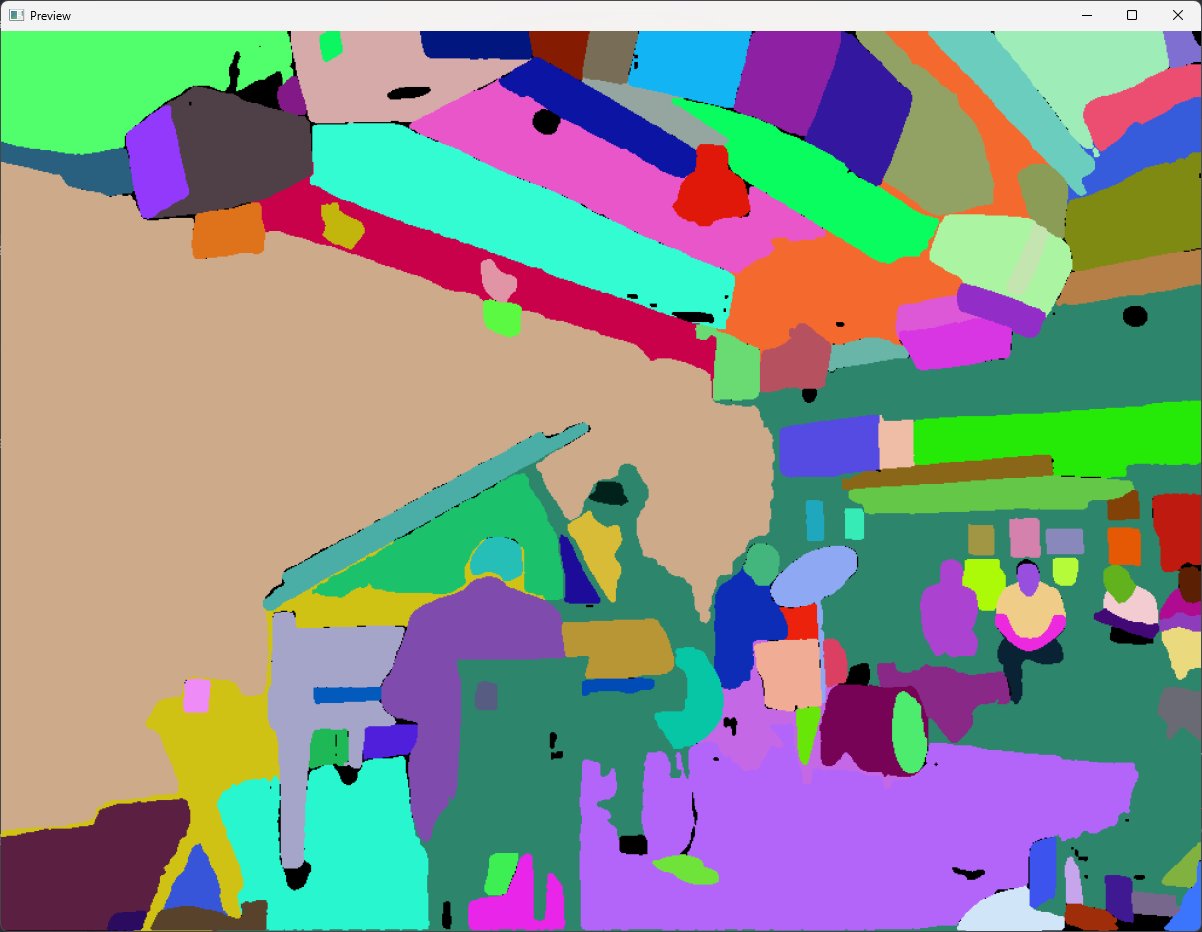
Another issue with the segmentation is that there seems to be long strands around objects. For example, the
model highlighted the edge of the grand piano lid, the pianist’s ears, and a table next to the piano as one big
segmentation in yellow.

While it doesn’t make much of a visual impact in this specific image, I found that it can be detrimental in
others. To fix this, I erode each segmentation five times then dilate it five times. This preserves the core
structure while removing any strands.
Now all segmentations are disconnected, which is much better!
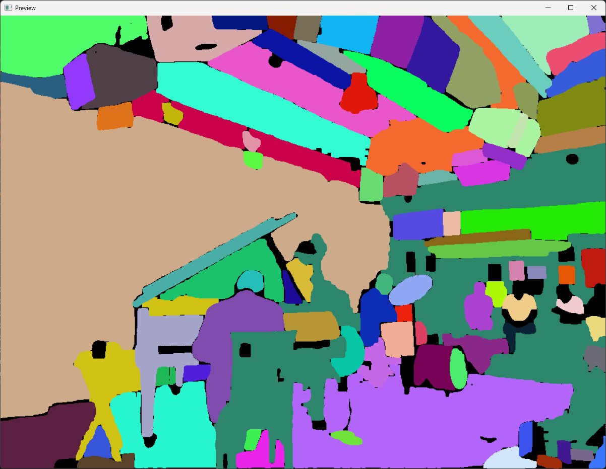
One final task is to set each black pixel to the color of the closest non-black pixel. This fills in the holes
we just created.
The new segmentations look pretty good! With these segmentations you get the following image:
I think this yields a minor visual improvement.
Making the colors pop
The current looks decent, but it can be improved by enhancing the colors. I use two tricks to make the colors pop.
The first technique may be obvious, but I just increase the saturation of the original image. I find increasing it by 50% (scale=1.5) works well despite being a very high value for regular images.
The second technique I employ is to take the median color instead of mean for every region. I suspect this works well since it asks “what is the dominant color” instead of “what is the average color,” which prevents two very different colors from averaging out.
Here’s the result with both techniques applied.

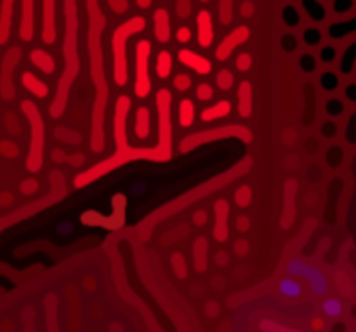
Aaah! Astonishing amounts of aliasing are apparent!!!
Attentive audiences are aware of an abundant aliasing anomaly. Okay, I’ll stop. But the edges of each region are
very jagged. This is obvious if you zoom in.
In computer graphics, this phenomenon is called aliasing, and occurs when there’s no subpixel smoothing.
 Diagram showing how aliasing occurs when there is no subpixel smoothing (GeeksForGeeks).
In my image processing pipeline, aliasing forms when I create a binary threshold of the blurred-and-sharpened image, which creates harsh boundaries. There’s a few ways to fix this.
The most intuitive method is to upscale the input image by, say, four times, then downscale the final result. This effectively keeps subpixel information but is very computationally expensive due to the O(n^2) time complexity.
Following this line of thinking, I tried using an AI upscaling model to increase resolution, then downscaled back to the original resolution. However, the edges were still jagged-looking after this process.
Instead, I take a simpler approach. Since the image consists of several solid-color regions, we can identify boundary pixels between regions and selectively smooth those. I compute the edges by finding where the morphological gradient is nonzero (OpenCV’s morphologyEx function does a lot of the heavy lifting). Then, I blur the entire image with a gaussian blur of standard deviation = 1.0 pixels. Finally, I set the color of each edge pixel with the corresponding color from the blurred image. This isn’t a ‘true’ antialiasing technique seen in computer graphics, but it gets the job done.
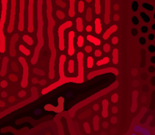
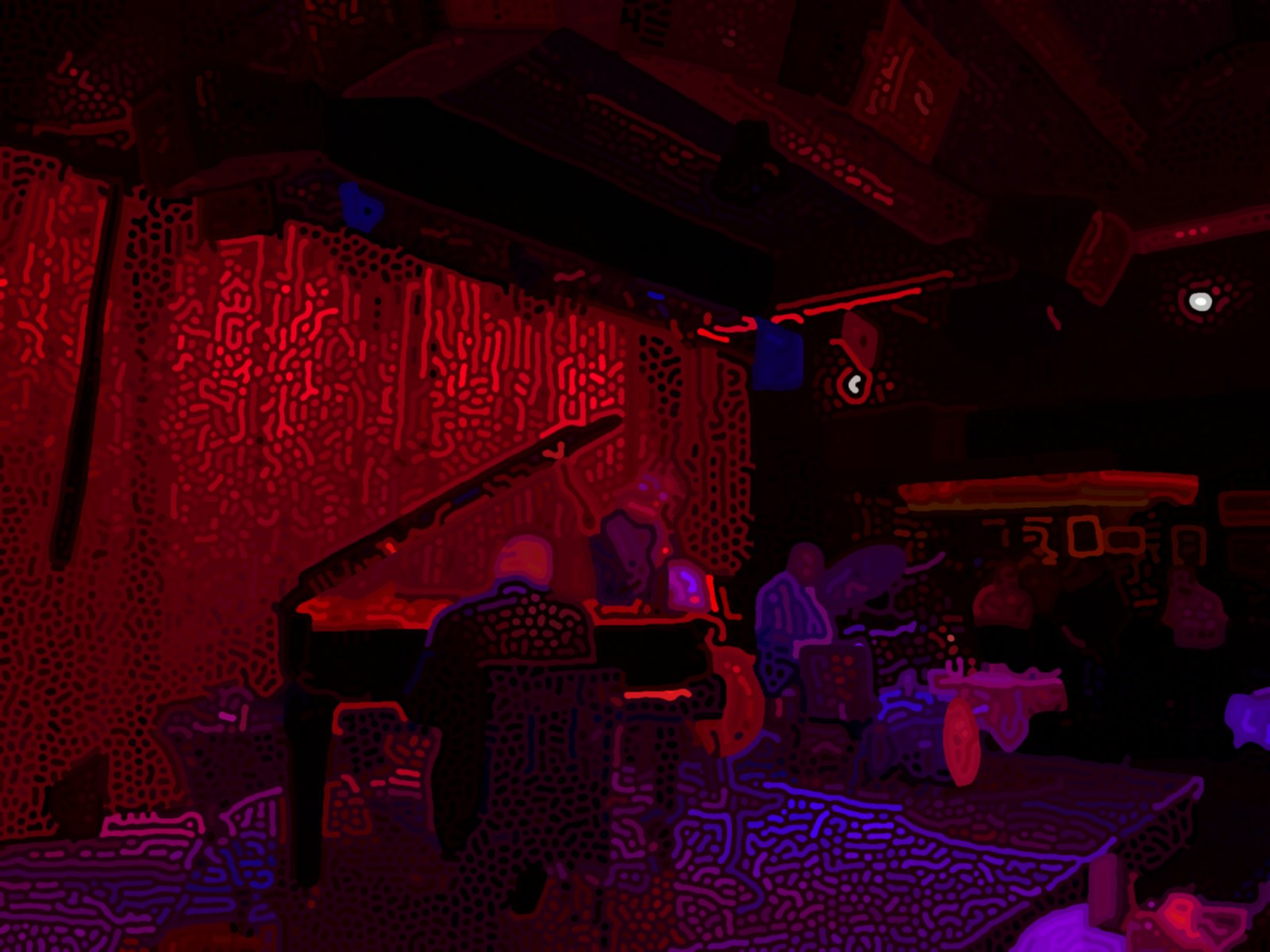
Here’s the image after antialiasing, zoomed in on a small section. Notice how the edges are much smoother.
Here's the full image.
Limitations and Future Work
The largest limitation with this project is the processing time of each image, which makes it inconvenient to fine-tune parameters or make small modifications. After a lot of optimization work, I was able to get processing time down to around 5 minutes. By far, blurring and sharpening the image is the largest contributor to the long processing time. Since each segment is blurred and sharpened individually, processing time scales approximately linearly with the number of segmentations. More intuitively, image processing time increases as images get more complex.
Another issue is with the segmentation. There are still artifacts or segmentations that shouldn’t exist. While writing this article, I noticed that increasing image saturation increases the number of artifacts. I’m unsure why this happens, since I’d imagine that the SAM training data would have been augmented such that it generalizes to cases like these. In future projects where I work with image segmentation, I’ll make sure to apply effects like saturation only after segmentation. But for this project, I came to a workaround where I manually specify several segmentations to remove. This means that the pipeline isn’t fully automatic.
Conclusion
I love the organic squiggles that this pipeline produces from just a few simple rules. From this project, I learned that I can extend image processing and computer graphics techniques far beyond simply rendering 3D scenes or scientific visualization, and I can use unorthodox techniques to make something beautiful.